
Introduction
Mel spectrogram is an audio analyzing technique which is predominantly applied to raw audio form as a preprocessing step before passing to any model for predictions. For example, speech-to-text models’ input raw audio is converted into mel spectrogram before passing to the model.
In general, mel spectrogram is a kind of visualization technique which takes into account how the human ear perceives audio frequencies during this low dimensional conversion process. Compared to the raw audio waveform and the more natural way humans perceive audio, these are all the predominant reasons we prefer audio in mel spectrogram form.
To fully understand how this conversion process occurs, what exactly is going on under the hood, and why we need this conversion, we need to understand a few other related concepts and techniques surrounding audio in general.
How Audio is Represented Digitally
In a physical sense, audio signals are continuous signals, but we usually represent this audio in discrete form when we represent it digitally. It is basically a list of numbers, usually 16-bit integers (if it’s a .wav file).
Each number in this list basically records the amplitude (strength of the physical sound waves) value captured by the microphone at various time points.
Sampling Rate
Now here, one parameter comes into the picture, which is how many samples the microphone should record in a given time period. For example, if our microphone records a lot of samples per second, then our audio quality would be much better, but there is a limit. This is usually 22k samples per second or 44k samples per second. These rates are enough to capture most of the audio frequency and quality. This rate is called the sampling rate.
Nyquist Theorem (Mathematical Guarantee)
Now another question comes up: why do these choices usually work, like 22k samples per second or 44k samples per second? There is one famous mathematical theorem called the Nyquist theorem, which provides strong theoretical guarantees. It says that if you want to capture higher frequencies, then your sampling rate should be 2 times the highest frequency you are trying to capture.
$$f_{max} = \frac{f_s}{2}$$
Where: $$\begin{aligned} f_{max} &= \text{highest frequency (Nyquist frequency)} \ f_s &= \text{sampling rate (Hz)} \end{aligned}$$
Usually, the human hearing range is 20 Hz to 20 kHz, so a sampling rate of 40 kHz will capture up to 20 kHz. This is enough for most cases. Sometimes music requires a slightly higher frequency range, so accordingly, a higher sampling rate is required.
Notational Meaning Difference
There is a slight notational difference here. Hz means different things when we talk about frequency and sampling rate. When we say 40 kHz, we are talking about 40k samples per second, and when we say 40 kHz in frequency, we are talking about cycles per second.
Time Domain Signal
Now this array of signal captures all required information of the audio signal. We can transmit it and play it using a speaker. This is called time domain signal because it is basically a signal across the time.
Frequency Domain Signal
One of the interesting and key ideas is that we can pick a particular instant in time and take the samples from that instant to check what are all the frequencies available.
This is done through another cool mathematical technique called Fourier transform which takes the samples of the audio at a particular instant in time and gives all the available frequency information at that instant. To be exact, it will give all the frequencies with their magnitude and phase information (usually complex numbers).
Of course, the maximum frequency it can extract is bound by Nyquist theorem, basically sampling rate / 2 is the maximum frequency we can extract.
Spectrogram
Now if we take this frequency information across different time instants, we will get frequency information at each instant of time across the time axis. This is called spectrogram.
We usually do two additional transformations on this spectrogram.
Taking only amplitude value. Fourier transform returns frequency value as a complex number which contains both amplitude and phase information of each frequency. Usually, we discard phase information and only keep amplitude information. This is done by taking the Euclidean norm of the real and imaginary parts.
Final transform is converting this amplitude value to decibel value, basically taking each amplitude value and taking the log of it. The reason seems to be that this closely matches how humans perceive the audio amplitude. To be exact, the following is the transformation formula.
$$\text{dB} = 20 \log_{10}\left(\frac{|A|}{A_{\text{ref}}}\right)$$
Where: $$\begin{aligned} \text{dB} &= \text{amplitude in decibels} \ |A| &= \text{absolute value of amplitude} \ A_{\text{ref}} &= \text{reference amplitude value} \end{aligned}$$
$$\text{dB} = 10 \log_{10}\left(\frac{|X(f)|^2}{X_{\text{ref}}^2}\right)$$
Or equivalently: $$\text{dB} = 20 \log_{10}\left(\frac{|X(f)|}{X_{\text{ref}}}\right)$$
Where: $$\begin{aligned} X(f) &= \text{Fourier transform at frequency } f \ |X(f)| &= \text{magnitude of the transform} \ X_{\text{ref}} &= \text{reference value} \end{aligned}$$
Mel Spectrogram
The spectrogram we have seen so far gives information about each instant, what are all the frequencies, and how it changes across the time.
There is another interesting fact: humans can’t very well differentiate between higher frequencies the way they do in lower frequency ranges. Basically, human frequency perception kind of follows a logarithmic function which implies if we take one instant of spectrogram frequency information, they usually have linear spacing, meaning 20 Hz, 40 Hz, 60 Hz, etc. (in this example 20 Hz apart). But as we move to higher frequency ranges, the human ear can’t distinguish this. Meaning the human ear can distinguish the difference between 20 Hz and 40 Hz but it can’t between 12 kHz and 12.20 kHz, even though the same space between both frequencies. So there is a lot of unnecessary frequency information (in terms of human perception point of view).
Which implies we can group a lot of the frequency based on this idea. This is done by first picking a set of frequency bands, usually 80 bands, which basically focus on different frequency ranges from 0 to max frequency. Each frequency band will have a set of weights which tries to capture human perception. Lower frequency weights will be mostly zero weights for far away frequencies and less weights for nearby frequencies. In higher frequency bands, weights will be dispersed because there we can combine a lot of frequencies.
This mel spectrogram process might not be obvious but when we go through the full code it will get clarified. But for now, it’s kind of a dimensionality reduction technique on spectrogram which takes into account how humans perceive sounds.
Code
Let’s do the full conversion process in code to see what exactly is going on. For most of the audio processing, let’s use a library called librosa which contains a lot of useful utility functions to work with the audio data and along with some sample audio data to work with.
First, let’s import required libraries and let’s use libri1 sample audio from librosa library which is basically human voice.
import librosa
import numpy as np
import matplotlib.pyplot as plt
import IPython as ipy

audio, sr = librosa.load(librosa.ex('libri1'))
In the above code, sr is a sampling rate and audio is our actual audio data which is a 1-dimensional array of numbers.
Following is the original audio.
Setup FFT Parameters
n_fft = 1024
hop_length = 512
Frequency Resolution
We know maximum frequency possible by Nyquist theorem is sampling_rate/2, so FFT can produce up to sampling_rate/2 frequency. Another fact is FFT algorithm produces symmetric values so only n_fft/2 bins are unique frequency bins. FFT algorithm works by evenly spaced frequency bins, so the spacing becomes (sampling_rate/2) / (n_fft/2) = sampling_rate/n_fft.
frq_resolution = sr/n_fft
print(f'frq resolution: {frq_resolution:.0f} Hz')
Time Resolution
1/sampling_rate will tell us spacing between individual sample points. n_fft * (1/sampling_rate) will tell us the time bracket the FFT instance occupies.
time_resolution = n_fft/sr
print(f'time resolution: {time_resolution*1000:.0f} ms')
There is a trade-off here. If we increase the time resolution, then we have to sacrifice the frequency resolution. So balance is required.
Frequency Bins Calculation
freq_bins = (n_fft//2) + 1
print(f"frequency bins: {freq_bins}")
Time Frame Calculation
How many time frames for the given audio signals after STFT. This is like convolution kernel operation.
total_time_frame_points = int((1+(len(audio)-n_fft)/hop_length))
print(f'estimated total time frame points: {total_time_frame_points:.0f}')
Short-Time Fourier Transform (STFT)
D = librosa.stft(audio, n_fft=n_fft, hop_length=hop_length)
print(f"stft output: {D.shape} = (frq_bins, time_frame_points)")
Amplitude Extraction
STFT contains both amplitude and phase information. Usually we take only amplitude information and discard the phase information. There is some subtlety here - np.abs for real part works just by taking normal abs, but if it’s a complex number, in this case it will calculate abs by taking Euclidean norm of the real and complex parts. Equivalent in PyTorch would be the following: x = torch.tensor([D[1][0].real, D[1][0].imag]) torch.sqrt(x.pow(2).sum(-1))
Amplitude is the strength of each frequency bin which is the one visualized in spectrograms.
D_amp = np.abs(D)
Logarithmic Transformation
Taking log of these amplitude values gives values that are more suitable to how humans perceive audio and relative difference between different frequency strengths. It won’t be exact log but close enough (actual formula will look like: 20 * log10(amplitude / reference)). The ref=np.max is basically used to normalize the audio to 1 range and take the log which shifts the values to negative side and max value will be 0, and this is done for conventional reasons.
S_db = librosa.amplitude_to_db(D_amp, ref=np.max)
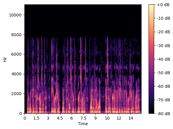
Display Spectrogram
librosa.display.specshow(S_db, x_axis='time', y_axis='hz', hop_length=hop_length)
plt.colorbar(format='%+2.0f dB')
plt.show()
Audio Reconstruction with Griffin-Lim Algorithm
If we want to convert this spectrogram back to the original audio signal, we face one caveat: during amplitude calculation we discarded the phase information. Phase information is crucial for the reconstruction.
One classical way to estimate that missing phase information is using an iterative algorithm which works like this:
- Assign random phase for the magnitude
- Calculate inverse short time Fourier transform (ISTFT) which will give audio signal
- Now calculate spectrogram from this new audio signal
- Compare the magnitude with original magnitude (kind of loss)
- Now estimate the new phase which reduces this loss
- Repeat this until loss is low
This algorithm is called the Griffin-Lim algorithm.
D_amp_reconstructed = librosa.db_to_amplitude(S_db)
reconstructed_audio = librosa.griffinlim(D_amp_reconstructed, n_iter=32,
                                         hop_length=hop_length,
                                         win_length=n_fft)

print(f"reconstructed audio shape: {reconstructed_audio.shape}")
ipy.display.Audio(reconstructed_audio, rate=sr)
You can hear that the reconstructed audio is not exactly the same as the original. This is because the phase information was estimated rather than preserved from the original signal. The Griffin-Lim algorithm provides a reasonable approximation, but there will always be some differences compared to the original audio.
Mel Spectrogram Generation
For mel spectrogram we have to take STFT output and convert to amplitude and take the power (which basically squares all the values). The reason why we take square is we want energy which is square of the amplitude. The reason why we need energy instead of amplitude is because human perception is better with power than amplitude.
from librosa.filters import mel

power_sepc = np.abs(D)**2
print(f"power spec shape: {power_sepc.shape}")
Mel filter bank is basically dimensionality reduction of the power spectrogram. These filters are created as follows:
- We take 80 evenly spaced points from fmin=(0) to fmax= sr/2
- Note these evenly spaced points are in log scale (exact formula: 2595 * log10(1 + hz/700))
- Now take these log scale 80 points to linear scale (exact conversion formula: 700 * (10^(mel/2595) - 1))
- This will be the center points for the filters in our frequency bins
- These filter values are peak at the center point and low at the edges like triangle
- Then we apply this filter across frequency bins dimension to get the final bin value
Basically lower frequency weight reduction will be steep because human perception in lower frequency range is good but higher frequency weight reduction will decrease slowly because in higher frequency range human perception of distinction becomes hard.
n_mels = 80
mel_filterbank = mel(sr=sr, n_fft=n_fft, n_mels=n_mels, fmin=0, fmax=sr/2)
print(f"mel filter bank shape: {mel_filterbank.shape}")

mel_spectogram = np.dot(mel_filterbank, power_sepc)
print(f"mel spec shape: {mel_spectogram.shape}")
Let’s convert back to dB scale. This is to match human loudness perception.
# this to match human loudness perception matching
mel_S_db = librosa.power_to_db(mel_spectogram, ref=np.max)

librosa.display.specshow(mel_S_db, x_axis='time', y_axis='mel', sr=sr, hop_length=hop_length)
plt.colorbar(format='%+2.0f dB')
plt.tight_layout()
plt.show()
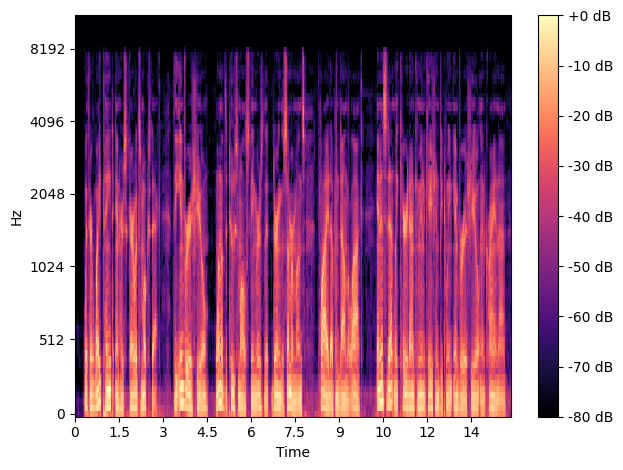
Figure: Mel Spectrogram with 80 mel bands. Notice how the frequency axis is now non-linear with more resolution in lower frequencies.
You can see how the Mel spectrogram differs from the regular STFT spectrogram we generated earlier. The Mel spectrogram has more resolution in the lower frequency ranges, which better matches human perception of sound. This is why Mel spectrograms are commonly used in speech recognition and music analysis applications.
Mel Spectrogram Inversion
Now let’s try to convert our mel spectrogram back to audio:
# power to db
mel_power = librosa.db_to_power(mel_S_db)

# mel filterbank which is used for the conversion.
mel_fb = librosa.filters.mel(sr=sr, n_fft=n_fft, n_mels=n_mels)

# take inverse of the mel.
# this will be less accurate as after mel conversion we lost some of the original information.
mel_inverse = np.linalg.pinv(mel_fb)
linear_spec_approx = np.dot(mel_inverse, mel_power)
print(f'linear spec approximate shape: {linear_spec_approx.shape}')

# power can't have negative values. so clip it.
linear_spec_approx = np.maximum(0, linear_spec_approx)


# this reconstruction may not be as accurate like the original direct spec to audio
# conversion because we lose information when we do this mel conversion.
mel_reconstructed_audio = librosa.griffinlim(linear_spec_approx, n_iter=32, hop_length=hop_length,
                                             win_length=n_fft)
ipy.display.Audio(mel_reconstructed_audio, rate=sr)
Notice how the audio quality from the Mel spectrogram reconstruction is generally lower than the reconstruction from the original STFT. This is because the Mel transformation is a dimensionality reduction process - we compress the frequency information from the full STFT bins (which was 513 frequency bins) down to just 80 Mel bands.
The process involves:
- Converting our dB scale Mel spectrogram back to power
- Getting the original Mel filterbank matrix
- Computing the pseudo-inverse of the Mel filterbank
- Using the pseudo-inverse to estimate the original linear spectrogram
- Ensuring all values are non-negative (power can’t be negative)
- Using Griffin-Lim algorithm to estimate the phase and reconstruct the audio
The Mel transformation deliberately discards information that isn’t perceptually significant to humans, making it excellent for tasks like speech recognition but less suitable for high-fidelity audio reproduction.
References
Wikipedia. “Nyquist–Shannon sampling theorem.” [Online]. Available: https://en.wikipedia.org/wiki/Nyquist%E2%80%93Shannon_sampling_theorem
Hugging Face. “Audio Course - Introduction.” [Online]. Available: https://huggingface.co/learn/audio-course/chapter0/introduction
3Blue1Brown. “But what is the Fourier Transform? A visual introduction.” YouTube. [Online]. Available: https://youtu.be/spUNpyF58BY
Librosa Documentation. [Online]. Available: https://librosa.org/doc/latest/index.html